The Mathematics of Snakes and Ladders

Many of us have at some point played the childhood game of Snakes and Ladders. Although there are no decisions to make, there is still quite a bit of mathematical structure to the game, which is useful in understanding the positional aspects of game theory, and probability theory in general.

A typical board is shown in Figure 1. Players start at square 0 (off the board), and in turn throw a 6-sided die and move the given number of spaces. If they land on a snake they go down to the bottom, and if they land on a ladder, they ascend to the top. The winner is the first player to reach square 100, but this requires an exact throw.

Figure 1: A typical Snakes and Ladders board. (Image may be subject to copyright.)

Like much of game theory, even simple games can pose some interesting questions:

1. 1. What is the maximum number of throws required to reach the finish square?
2. 2. What is the minimum number of throws required to reach the finish square?
3. 3. How many throws, on average, does it take to reach the finish square?
4. 4. Would you rather be on square 81 or square 53? Does it matter who goes next?
5. 5. In a two-player game, what is the probability that the player who starts first wins?
6. 6. In a game of three players, at positions 10, 15 and 27, who act in that sequence, what’s the probability that each player wins?
7. 7. In a ten-player game, what is the probability that the player who goes last wins?
8. 8. How many rounds does a 2-player game last, on average?
9. 9. How many rounds does a 3-player game last, on average?
10. 10. With three players at positions 10, 15 and 27, how many more rounds is the game expected to last?
11. 11. What’s the probability that you reach the finish in the minimum number of throws?
12. 12. What’s the probability that you need more than 100 throws to reach the finish?
13. 13. What is the probability of landing on square 80?
14. 14. What is the expected number of times you will land on the big ladder on square 28, before reaching the finish?
15. 15. Which are the least and most likely squares you will land on (apart from the start and finish)?
16. 16. Which square will you land on the most often before reaching the finish?
17. 17. What are the fairest starting positions for 10 players? (Assume that players don’t all have to start from the same square.)

Do try these questions yourself first, but you’ll need a computer to actually calculate the answers. There's also a bit of subtlety in the implementation which I won't go into but can be seen in the source code.

For all of these questions, precise answers can be formulated. This is much more insightful than doing a simulation to approximate the answers, although simulation is useful to validate the results.

Source code is here: http://www.calumgrant.net/projects/snakesandladders. I wrote this because I haven’t seen any other analyses of Snakes and Ladders, and it turned out to be a lot more interesting than I expected.

Answers
1-Unlimited, 2-7, 3-35.5432, 4-81,no, 5-0.509027, 6-0.280842,0.335736, 0.383422, 7-0.0907991, 8-24.421, 9-20.4108, 10-17.9524, 11-0.00173611, 12-0.0170009, 13-0.493964, 14-0.464519, 15-2,45, 16-99, 17-33,34,37 35,17,38,18,19,20,39.

Question 1

What is the maximum number of throws required to reach the finish square?

On most boards, such as the board in Figure 1, there is no upper bound on the number of throws to finish. It’s possible to carry on playing forever.

Question 2

What is the minimum number of throws required to reach the finish square?

We can express the minimum number of throws T for each square s as min(T). This can be expressed as as 1 + the minimum number of throws from each square we can land on from s.

     min(T(s)) = 1+min[1<=d<=6](min(T(move(s,d))))          (2)

     min(T(100)) = 0

where move(s,d) is the square we end up on if we throw a d on square s.

min(T) can be computed in various ways. For example, we can iterate over an array, or treat the squares as a graph and use a "single-source shortest path” algorithm.

The plot of min(T) for each square is shown in Figure 2.

Figure 2: The minimum number of throws remaining for each square.

The answer is min(T(0)), the minimum distance from square 0, which is 7.

Question 3

How many throws, on average, does it take to reach the finish square?

The expected number of remaining throws E(T(s)) for a square s is given by

     E(T(s)) = 1 + sum[1<=d<=6]E(T(move(s,d)))/6          (3)

     E(T(100)) = 0

Equation 3 comes from the sum over conditional probabilities, for each possible value of the die d, which have equal probability of 1/6.

This yields a set of linear equations which can be solved exactly using a linear equation solver. Another approach is to apply Equation 3 repeatedly on an array of E(T) initialised to 0, until the values in the array converge. This is correct because the values of E are monotonic so will stabilise by virtue of the Fixed Point Theorem.

The plot of E(T) is shown in Figure 3. The downward spikes are ladders, and the upward spikes are snakes. Squares 80 and 100 are at zero because they reach the finish.

Figure 3: The expected number of throws remaining for each square.

Calculating the expected number of throws from the start square = E(T(0)) = 35.5432.

Question 4

Would you rather be on square 81 or square 53? Does it matter who goes next?

Equation 3 gives

     E(T(53)) = 23.7185

     E(T(81)) = 23.6829

Thus, it seems that square 81 is better, because it is 0.0356 throws ahead - a tiny margin. The next player has one throw in hand, so it would seem to be at an advantage. But actually this isn’t true, because E(T) doesn’t tell the whole story.

The probability of the first player winning P_wins(a,b), when the players are in positions a and b, is given by

     P_wins(a, b) = sum[1<=d<=6](1-P_wins(b, move(a,d)))/6     (4)

     P_wins(100, b) = 1

Equation 4 comes from the sum of conditional probabilities, that for each throw of the dice, the other player doesn't win. Equation 4 yields a large set of linear equations, which can be solved using a linear equation solver. This yields

     P_wins(53,81) = 0.487661

     P_wins(81,53) = 0.535979

Thus the player on square 81 is more likely to win, irrespective of who goes first.

Intuitively, the player with the smaller number of expected moves remaining should be more likely to win. It turns out that there is an approximately linear relationship between the delta (difference) in the number of throws remaining, and the probability of winning a 2-player game. Figure 4 shows a plot of this, computed for all pairs of squares. The graph is not symmetrical because there's always a slight advantage in going first, giving an average bias of about 0.9% to the player first to act.

Figure 4: The difference in expected throws remaining, versus the probability of winning.

Figure 4 gives a quick way to estimate the probability of winning. Look up the expected values E(T) for each player in the Appendix, and P_wins is approximated by 0.018x+0.5094, or about 2% per throw.

Question 5

In a two-player game, what is the probability that the player who starts first wins?

Using the results from Equation 4, 

     P_wins(0,0) = 0.509027

I.e. the advantage of going first = 0.509027 - 0.5 = about 0.9%. The reason this is so low is because it’s relatively unlikely for two players to reach the finish square in exactly the same round.

Question 6

In a game of three players, at positions 10, 15 and 27, who act in that sequence, what’s the probability that each player wins?

Unfortunately Equation 4 is limited to 2 players, and calculating every state would become computationally expensive as there are 100^n game states for n players.

E(T) doesn't tell the whole story about who will win or give information about the distribution of throws remaining. We actually need to compute the random variable T(s) (representing the number of throws remaining at any any given square s).

The cumulative distribution function F(s;t) gives the probability that the finish square has been reached within t throws from square s.

     F(s; t) = sum[1<=d<=6](F(move(s,d)), t-1) / 6             (6a)

     F(100; t) = 1

     F(s; 0) = 0      for s!=100

     f(t) = F(t) - F(t-1)

Equation 6a uses the sum over conditional probabilities that you will reach the finish in t throws from s, if you can reach the finish in t-1 throws from any square reachable by s. Since F(s;t) is defined only in terms of F(s;t-1), we can iterate through t to calculate F. The probability density function f is the difference between sequential values of F.

Figure 6a shows a plot of f for various values of s, and Figure 6b shows the corresponding plots of F. The plot of f(0) is flat for the first 6 throws because it’s impossible to reach the finish in less than 7 throws.

Figure 6a: The probability distribution f of the duration of a game T, from the start (square 0), square 50 and square 90.

Figure 6b: The cumulative distribution F for the duration of a game T, from the start (square 0), square 50 and square 90.

F can be used to figure out who will win in the general case (unlike Equation 4 which is limited to the 2-player case). Assuming the players are in positions p_1 ... p_2,

     P(player 1 wins)

          = sum_t( P(Player 1 wins in t throws) * P(no other player wins in < throws) )

          = sum_t( f(p_1; t) * (1-F(p_2; t-1)) * … * (1-F(p_n; t-1) ) )                  (6b)

Note that it is very important that player 1 goes first, otherwise we would need to adjust each term to (1-F(p_i; t)) for all players i acting before the current player.

Thus we can plug in the values 10, 15 and 27 into Equation 6b, to get

     P(player 1 wins) = 0.280842

     P(player 2 wins) = 0.335736

     P(player 3 wins) = 0.383422

These add up to 1.

Question 7

In a ten-player game, what is the probability that the player who goes last wins?

This is evaluated from Equation 6b, to 0.0907991.

Figure 7a shows the probability of each position winning a multiplayer game, calculated using Equation 6b, where as expected, the players who act in early position are at an advantage. The advantage to the first player is consistently around 0.9%, and the last player has the same disadvantage.

 

Figure 7a: The probabilities for each player winning a multi-player game.

Why is the positional advantage consistently around 0.9%, irrespective of the square and the number of players? This actually comes from the probability that two players finish in the same round

     sum[t>0](P(T(p_1)=t and T(p_2)=t)

     = sum[t>0](f(p_1;t)*f(p_2;t))          (7)

where p_1 and p_2 are the respective positions of the players. Calculating Equation 7 from square 0, the probability of both players finishing in the same round = 0.0180536 ~= 1.8%. This is also the approximate advantage per throw in hand from Figure 4, as well as the difference in winning probabilities in a 2-player game (see Question 5.)

Proof:

     P(wins in position 1) - P(wins in position(2)

     = sum[t>0](f(t).F(t)) - sum[t>0](f(t).F(t-1))

     = sum[t>0](f(t) * (F(t) - F(t-1))

     = sum[t>0](f(t) * (F(t-1)+f(t) - F(t-1)))

     = sum[t>0](f(t) * f(t))

which is the same as Equation 7.

Figure 7b shows the probability of players finishing in the same round for each square, assuming they are both on the same square. As the number of expected throws remaining decreases, so the probability that both players finish in the same round increases.

Figure 7b: Probability of two players finishing in the same round for each square.

Question 8

How many rounds does a 2-player game last, on average?

The random variable T(0) defined in Question 6 gives the number of throws for one player to reach the finish. With 2 players, play stops as soon as one of the players reaches the finish, which is the minimum of two independent distributions T(0).

The cumulative distribution function (CDF) of the minimum of n identical distributions is given by

     F_n(t) = 1 - (1-F(t))^n          (8a)

The probability density function is as before

     f_n(t) = F_n(t) - F_n(t-1)

This new distribution is plotted in Figure 8.

Figure 8: Probability distributions of the number of rounds in a 1- and 2-player game.

The expected value of a distribution is given by 

     E(T) = sum_t(t*P(t=T)) = sum_t(t*f(t)),      (8b)

which is computed to be 24.421. As expected, the number of rounds player by 2 players is smaller than the number of rounds played by 1 player (35.5432) because the game stops as soon as one player reaches the finish.

Question 9

How many rounds does a 3-player game last, on average?

The same approach as Question 8 is used, with the minimum of 3 distributions. The new distribution is plotted in Figure 9a. The expected value of this distribution is calculated using Equation 8b, which evaluates to 20.4108. As expected, this is fewer rounds than with 2 players.

Figure 9a: Probability distributions of the number of rounds of a 1-, 2-, 3-player game.

Figure 9b shows the expected number of rounds plotted against the number of players, which is calculated by applying Equation 8b for each number of players. It starts with the value E(T(0)) = 35.5432 and decreases asymptotically to min(T(0)) = 7, because no matter how many players there are, a game cannot be finished in fewer than 7 rounds.

Figure 9b: The expected number of rounds in a game, plotted against the number of players.

Question 10

With three players at positions 10, 15 and 27, how many more rounds is the game expected to last?

A similar approach to Question 8 is required, but this time we are taking the minimum of 3 different independent distributions, because each square has its own distribution of remaining throws.

     F(t) = 1 - (1-F(10;t))(1-F(15;t))(1-F(27;t))

This new distribution is plotted in Figure 10, and the expected value of this distribution (using Equation 8b) = 17.9524.

Figure 10: Probability distribution of remaining rounds with players at squares 10, 15 and 27.

Question 11

What’s the probability that you reach the finish in the minimum number of throws?

We can answer this from the distribution for T in Equation 6a. The minimum number of throws=7, and F(7) = f(7) = 0.00173611.

Question 12

What’s the probability that you need more than 100 throws to reach the finish?

     P(T>100) = 1-P(T<=100) = 1-F(100) = 0.0170009.

Question 13

What is the probability of landing on square 80?

For this question, we need to figure out the probability of being on a particular square s on turn t.

     P(on square s on throw t) = sum[1<=d<=6](P(on square s0 on throw t-1) | s=move(s0,d))/6.     (13)

     P(on square 0 on throw 0) = 1.

Again we are using the sum of conditional probabilities to define the probability of one state (being on square s on throw t) in terms of the probabilities of other states. This type of calculation is called a “Markov chain” where the system (i.e. the state-space of the game) is in one of many possible states (in this case, parameterised by s and t), with probabilities of transition between them = 1/6 because there are 6 sizes of a die.

Since square 80 does not have any paths back to itself (it goes straight to square 100), we know that each of states P(s,t) are mutually exclusive, thus 

     P(lands on square 80) = sum[t>0](P on square 80 on throw t).

We can compute Equation 13 directly by iterating over t. The answer is 0.493964. I.e. half the time you win by the ladder on square 80, and the other half if you reach the finish via the top row on the board.

Question 14

What is the expected number of times you will land on the big ladder on square 28, before reaching the finish?

Unlike in the previous question, the Markov states are not independent, so we cannot simply add up the probabilities of landing on square 28. If you land on square 28, there’s a possibility that you end up back on square 28 again.

We can however limit the Markov chain defined in Equation 13, to only permit one visit to a particular square s. This is done by simply removing all transitions in the chain away from square s, and so

     P(lands on square s) = sum[t>0](P(first lands on square s on throw t)).

In fact, we can define the Markov chain from any starting square, allowing us to compute P(reaches s1 from s0) in general.

For example, P(reaches 100 from s0) is always 1, because you are guaranteed to reach the finish square if you play for long enough.

We need to figure out the distribution N_s of the number of times a particular square s is visited. We can interpret N_s as a variation of a geometric distribution, representing the number of failed attempts to reach square 100. A player either reaches s (with probability p), or reaches square 100 (with probability 1-p). When they are on square s, they either reach square s again (with probability q), or they reach square 100 (with probability 1-q).

     P(N = 0) = 1-p

     P(N = k) = p.(1-q).q^(k-1)          (14)

That is, if N=k then we reached square s from 0 (probability p), then reached ourselves k-1 times (probability q^(k-1)), then reached the finish (probability 1-q).

Figure 14a shows the values for p and q for each square, computed using the Markov chain.

Figure 14a: The probability of landing on each square at least once (blue) and the probability of landing on the square a second time (green), computed using a Markov chain.

Figure 14b shows the distribution of N for square 28, calculated using Equation 14. It falls away exponentially.

Figure 14b: Probability distribution of the number of times square 28 is landed on.

We could draw such a graph for any square on the board. Figure 14c shows the probability of landing on each square a given number of times, P(N_s=n), calculated using Equation 14.

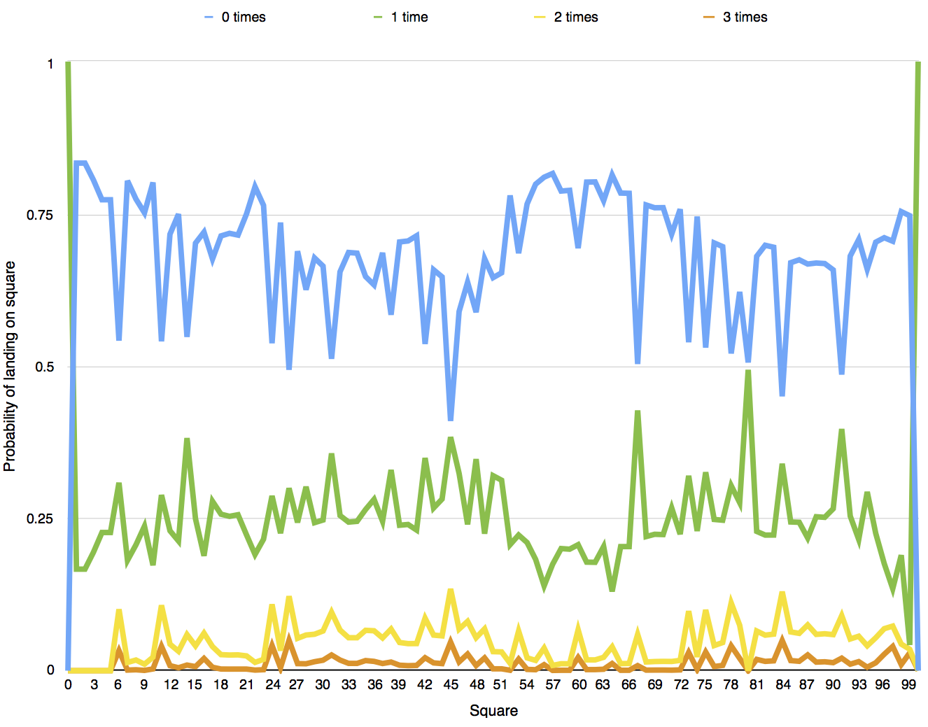
Figure 14c: The probability of landing on each square a given number of times.

Theorem 14: The mean of this distribution E(N) = p/(1-q).

Proof:

     E(N)   = sum[k>=1](k.p.(1-q).q^(k-1))

               = p.sum[k>=1]( k.(1-q).q^(k-1))

               = p.sum[k>=1]( k.q^(k-1) - k.q^k)

               = p.sum[k>=0]( (k+1)q^k - k.q^k)

               = p.sum[j>=0](q^j)

               = p/(1-q).

For square 28, we compute p = 0.37451, q= 0.193768, so by Theorem 14, E(N) = 0.38451/(1-0.193768) = 0.464519.

Question 15

Which are the least and most likely squares you will land on (apart from the start and finish)?

In this question we are only looking at p for each square to see if we landed on it or not. We can calculate p as P(reaches square s from 0) using the Markov chain from Question 14, to give a value of p for each square.

This gives the least likely square = 2 with p=1/6, the most likely square = 45 with p=0.590058.

Question 16

Which square will you land on the most often before reaching the finish?

This time we are looking for the square with the highest value of E(N). Calculating E(N) for each square using Theorem 14, and taking the maximum, gives the square with the most visits = 99 with 1.51811. This is because when you are on this square, you are likely with probability 5/6 to visit it again in the next throw (because you have to throw a 1 to finish.)

Figure 16 shows E(N) for each square.

Figure 16: The expected number of visits E(N) to each square in one game.

Question 17

What are the fairest starting positions for 10 players?

The problem as shown by Figure 7a is that players who are in early position get an unfair advantage. So we need to find a fairer set of squares, where the probability of winning for each player is as close to 1/10 as possible. Since there are 100^10 =10^20 different possible starting positions, it’s not feasible to do an exhaustive (“brute-force”) search. We also need to define what's meant by “fair."

These problems don't exist for the 2-player case. By searching every value of P_wins (calculated in Question 4), we find that the starting positions with probabilities closest to 0.5 is squares 39 and 22, with probabilities 0.49994 and 0.50006. Of course it would look a bit weird to start from these squares!

This is an example of an optimisation problem where we need to search a large complex space for the optimum solution. The strategies I investigated were:

1) Pruning the search space, to reduce the number of positions we analyse from 10^20 to something much smaller.

2) Stoichastic methods, for example to guess solution and iterate to a better one.

In order the prune the search space, we can use two insights:

Insight 1: The positions in the solution are likely to have a similar value of E (calculated in Question 3.)

Insight 2: For a partial solution, the first n players should be "fair", irrespective of the values of the other positions.

Both of these insights provide a way to exclude large numbers of potential solutions without evaluating them all explicitly, but leave open exactly what thresholds to use. 

After experimentation, the best solution I could find is: 33, 34, 37, 35, 17, 38, 18, 19, 20, 39 with standard deviation 0.000571703. More details can be found in the source code. Figure 17 shows a plot of the winning probabilities for each player, calculated using Equation 6b. Like the 2-player case, there isn’t a perfect solution.

Figure 17: Probabilities of each player winning in positions 33, 34, 37, 35, 17, 38, 18, 19, 20, 39.

To evaluate each solution for fairness I used the standard deviation of the probabilities (calculated using Equation 6b) - a perfectly fair position would have a standard deviation of 0. I also disallowed starting on the top of snakes or the bottom of ladders, mainly because these squares can't be landed on in normal play.

Stoichastic methods involve random sampling of the search space (which in this case is huge), plus the ability to locally optimise a solution, for example by adjusting one position at a time. This method also found the above solution, but overall seemed much less reliable.

The following table shows the results for different numbers of players. Nevertheless this is still an open question - maybe other solutions exist?

Number of players	Fairest position
2	39, 22
3	35, 26, 24
4	31, 33, 37, 38
5	30, 32, 17, 18, 20
6	30, 32, 33, 34, 35, 20
7	31, 32, 33, 34, 35, 38, 20
8	30, 32, 33, 34, 37, 35, 18, 19
9	31, 32, 33, 34, 37, 35, 38,18, 19
10	33, 34, 37, 35, 17, 38, 18, 19, 20, 39
11	30, 31, 32, 33, 33, 34, 37, 35, 38, 17, 18
12	30, 31, 32, 33, 33, 37, 34, 35, 38, 17, 18, 18

Table 17: The fairest positions for different numbers of players.

Conclusion

That’s it for now! I’ve exhausted the mathematical possibilities of Snakes and Ladders for now, and I hope the tour has been both accessible and interesting.

It turns out that we can derive precise answers for most of the questions we can ask of a game of Snakes and Ladders. Next time you’re playing Snakes and Ladders, you can now reel off interesting facts about each square, see who’s really ahead, and estimate your odds of winning.

Appendix

The following table contains computed values for some of the figures in this article. These values are only applicable for the board shown in Figure 1.

Square	Minimum throws remaining min(T)	Expected throws remaining E(T)	Completion %	Winning probability adjustment %	Probability of finishing in the same round %	Probability of landing (p) %	Probability of landing again (q) %	Expected number of visits E(N)	Visits by Monte Carlo E(N)
0	7	35.5432	0	32.3008	1.80536	100	0	1	1
1	6	31.1991	12.2221	40.575	1.804	16.6667	0	0.166667	0.166884
2	7	36.0292	-1.36721	31.3752	1.80598	16.6667	0	0.166667	0.166236
3	6	35.4548	0.248945	32.4693	1.81191	19.4444	0	0.194444	0.194488
4	6	33.6121	5.43321	35.979	1.8131	22.6852	0	0.226852	0.227304
5	6	35.5725	-0.0822114	32.2451	1.81245	22.6852	0	0.226852	0.226388
6	6	35.3918	0.426064	32.5892	1.81191	45.8211	32.6582	0.680425	0.680628
7	6	35.1843	1.00983	32.9844	1.81158	19.565	7.44933	0.211398	0.212512
8	6	34.9597	1.64174	33.4122	1.81161	22.5773	8.45734	0.246631	0.2471
9	5	32.0082	9.94588	39.0341	1.80273	24.8336	4.47104	0.259958	0.259816
10	7	35.1719	1.04472	33.0081	1.80288	19.8454	12.7869	0.227551	0.226548
11	6	34.7189	2.31934	33.871	1.80283	45.9289	37.2128	0.731501	0.732532
12	6	34.3079	3.47572	34.6538	1.80393	28.3364	18.9426	0.349584	0.349536
13	6	33.9394	4.51246	35.3557	1.80615	25.0372	14.9679	0.294444	0.29386
14	6	33.6121	5.43321	35.979	1.80935	45.208	15.5208	0.535137	0.536116
15	6	33.0615	6.98238	37.0278	1.82247	29.8098	16.3515	0.35637	0.356508
16	6	35.3918	0.426064	32.5892	1.83917	27.9983	32.6582	0.415765	0.41618
17	5	32.0006	9.96703	39.0484	1.83544	32.4128	14.2153	0.377839	0.37634
18	5	31.8418	10.414	39.351	1.83383	28.6225	10.245	0.318896	0.318352
19	5	31.7284	10.7329	39.5669	1.83349	28.1983	10.134	0.313781	0.314332
20	5	31.6485	10.9577	39.7191	1.83405	28.4871	10.1364	0.317004	0.317408
21	5	29.7577	16.2774	43.3205	1.81738	25.0151	10.8666	0.280648	0.280964
22	4	30.3402	14.6386	42.211	1.82683	20.5448	7.14363	0.221253	0.219348
23	4	30.6872	13.6624	41.5501	1.81568	23.6	8.57278	0.258129	0.259208
24	4	30.8885	13.096	41.1667	1.81523	46.2443	37.9585	0.745377	0.746348
25	4	31.0485	12.646	40.862	1.81836	26.4191	14.5726	0.309257	0.309632
26	4	31.169	12.3067	40.6323	1.8241	50.6056	40.8079	0.854939	0.85714
27	4	31.2491	12.0814	40.4798	1.83171	31.1289	21.818	0.398159	0.395384
28	3	20.999	40.9199	60.0033	1.91016	37.451	19.3768	0.464519	0.465216
29	6	32.769	7.80527	37.5849	1.91347	32.237	24.6171	0.427644	0.426368
30	5	32.0965	9.69743	38.8659	1.90021	33.5797	26.3435	0.455896	0.456448
31	5	32.0082	9.94588	39.0341	1.90612	48.8003	26.9027	0.667608	0.669336
32	5	31.8926	10.271	39.2542	1.91262	34.5031	26.1767	0.467374	0.467312
33	5	31.7295	10.7299	39.5649	1.91844	31.3426	22.1844	0.40278	0.402704
34	5	31.5231	11.3106	39.958	1.92522	31.4534	22.0582	0.40355	0.405772
35	5	31.3642	11.7576	40.2606	1.92832	35.2915	25.0406	0.470809	0.468088
36	4	28.0612	21.0504	46.5518	1.94352	36.6667	23.2919	0.478003	0.47792
37	6	31.4783	11.4365	40.0432	1.94117	31.397	21.902	0.40202	0.4042
38	6	31.1991	12.2221	40.575	1.94812	41.5718	20.7283	0.524422	0.523236
39	5	30.7509	13.4832	41.4288	1.94684	29.6123	19.3705	0.367264	0.368232
40	5	30.2847	14.7947	42.3167	1.95947	29.4499	18.4991	0.361344	0.361092
41	5	30.4111	14.4392	42.0761	1.93526	28.6024	19.2728	0.35431	0.355588
42	5	29.7577	16.2774	43.3205	1.97578	46.3619	24.6811	0.615542	0.616648
43	5	30.4665	14.2834	41.9706	1.91661	34.1804	21.8705	0.437484	0.43792
44	5	29.524	16.9351	43.7657	1.99045	35.3458	20.2836	0.443394	0.443964
45	4	28.0612	21.0504	46.5518	2.00464	59.0058	35.008	0.907893	0.907252
46	4	27.488	22.6632	47.6436	2.08662	41.0383	21.0793	0.519994	0.521984
47	4	31.169	12.3067	40.6323	2.28711	36.2262	33.7047	0.546436	0.548232
48	4	25.8376	27.3066	50.7871	2.36254	41.1458	15.5783	0.487384	0.484744
49	6	34.7189	2.31934	33.871	2.71689	32.3729	30.534	0.466025	0.465292
50	4	23.869	32.8452	54.5368	2.76238	35.4741	9.76064	0.393111	0.391412
51	3	19.2849	45.7423	63.268	2.97539	34.683	9.8511	0.38473	0.386036
52	5	24.0485	32.3401	54.1948	2.99579	21.9744	5.85699	0.233415	0.233832
53	5	23.7185	33.2687	54.8234	3.01402	31.46	29.2056	0.444385	0.440348
54	5	23.3858	34.2047	55.4571	3.03121	23.3726	10.0068	0.259716	0.258928
55	5	23.0577	35.1278	56.0821	3.04872	20.131	9.22639	0.221771	0.220616
56	5	23.7185	33.2687	54.8234	3.16363	18.9813	26.6376	0.258733	0.256224
57	4	22.2681	37.3494	57.586	3.17497	18.3697	4.92568	0.193214	0.1927
58	4	22.1426	37.7025	57.8251	3.23348	21.2575	5.69701	0.225417	0.225024
59	4	21.7383	38.8398	58.595	3.25974	21.1422	5.65066	0.224084	0.222912
60	4	21.3896	39.8208	59.2592	3.29177	30.6328	32.4877	0.453737	0.451312
61	4	21.089	40.6668	59.8319	3.33415	19.786	9.94258	0.219704	0.218804
62	3	20.7737	41.5537	60.4323	3.37495	19.7548	9.94306	0.219359	0.217904
63	3	20.4752	42.3936	61.0009	3.41927	22.8398	10.7537	0.255919	0.255048
64	4	21.3896	39.8208	59.2592	3.71724	18.6126	30.1249	0.26637	0.262968
65	3	19.3128	45.6641	63.215	3.95471	21.5882	5.64629	0.228801	0.22794
66	3	19.2975	45.7069	63.244	3.9631	21.628	5.79601	0.229587	0.228804
67	3	19.2849	45.7423	63.268	4.04499	49.6539	13.9386	0.576959	0.578504
68	2	18.8821	46.8756	64.0352	4.0272	23.5443	6.48519	0.251771	0.25064
69	2	18.6842	47.4326	64.4123	4.05157	23.9964	6.69127	0.257173	0.256788
70	2	18.6204	47.612	64.5337	4.11306	23.9811	6.82663	0.257382	0.256716
71	2	15.1073	57.4959	71.2251	4.18276	28.33	5.6542	0.300278	0.30014
72	2	19.2062	45.9639	63.418	4.4182	24.2385	7.53766	0.262145	0.261724
73	2	19.2095	45.9547	63.4117	4.82297	46.0793	30.5657	0.663639	0.662636
74	1	16.4653	53.6754	68.6386	6.0686	25.4291	9.83163	0.282018	0.281904
75	1	17.4963	50.7745	66.6747	5.41473	46.9618	30.6346	0.67702	0.677016
76	1	18.2378	48.6883	65.2624	4.99829	29.774	16.6074	0.357034	0.357108
77	1	18.7537	47.2369	64.2798	4.77477	30.3803	18.6917	0.373643	0.372936
78	1	19.0745	46.3345	63.6689	4.72228	47.9173	36.6062	0.755867	0.754336
79	1	19.2292	45.8993	63.3742	4.83408	37.8112	27.034	0.518203	0.518044
80	0	0	100	100	3.01719	49.3964	0	0.493964	0.493952
81	4	23.6829	33.3688	54.8912	2.71768	31.9694	28.4739	0.446961	0.446408
82	3	22.6868	36.1713	56.7885	2.88572	30.1589	26.1929	0.408618	0.407028
83	3	21.849	38.5284	58.3842	3.0355	30.4814	26.9409	0.417215	0.416628
84	3	20.999	40.9199	60.0033	3.23077	54.9615	38.1758	0.888997	0.889656
85	3	20.1573	43.2879	61.6064	3.48127	33.0222	26.0695	0.446666	0.44556
86	3	19.5169	45.0898	62.8263	3.71408	32.5435	25.1432	0.434743	0.4342
87	4	30.8885	13.096	41.1667	4.48449	33.2395	34.4646	0.5072	0.507272
88	2	16.71	52.9869	68.1725	4.61404	33.0701	23.5739	0.432706	0.432036
89	2	16.8223	52.6708	67.9585	4.47446	33.159	24.0729	0.436721	0.435412
90	2	15.8989	55.2689	69.7174	4.89473	34.2022	22.2628	0.439972	0.438912
91	2	15.1073	57.4959	71.2251	5.3765	51.3866	22.7749	0.665413	0.664176
92	2	15.6741	55.9014	70.1456	5.26552	31.9317	20.4873	0.401593	0.401732
93	2	19.2095	45.9547	63.4117	6.30315	29.2131	26.2421	0.396068	0.39522
94	1	11.5479	67.5104	78.0048	7.06861	34.0942	13.9182	0.396068	0.394964
95	1	17.4963	50.7745	66.6747	7.43353	29.6478	23.9725	0.389961	0.389016
96	1	10.3582	70.8576	80.2708	7.43353	28.917	39.2196	0.475761	0.476792
97	1	10.3582	70.8576	80.2708	7.43353	29.4965	54.3595	0.646278	0.643144
98	1	19.0745	46.3345	63.6689	9.09091	24.6316	23.0141	0.31995	0.319
99	1	6	83.1192	88.5718	9.09091	25.3018	83.3333	1.51811	1.52813
100	0	0	100	100	100	100	0	1	1